Previous: Spacetime Fundamentals

Next: Lorentz Transformations

2. Objects in Spacetime

Features Introduced

• The spacetime.physical.MovingObject type
• Object and spacetime animations using visualize.stanimate and visualize.stanimate_with_worldline
  • Animator objects
• The basic geom objects:
  • STVector
  • Line
  • Ribbon

---

We’ve already seen the STVector. Now let’s look at some other LorentzTransformable objects, and some other visualization tools at our disposal.

Let’s assume that we use the following parameters for all the plots in this module.

include_grid = True
include_legend = True
tlim = (0, 2)
xlim = (-2, 2)

One of the most common things we’ll want to plot is an object moving through space at a constant speed and direction. This is what the MovingObject is for. Let’s plot a stationary point object at x = 0.

stationary = phy.MovingObject(0, draw_options={'label': '$v = 0$'})
title='Stationary object'
p = vis.stplot(stationary, title=title, tlim=tlim, xlim=xlim,
    grid=include_grid, legend=include_legend)
p.save('2-objects_stationary_point.png')
p.show()

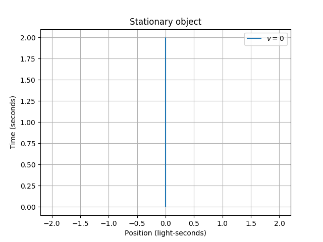
A stationary object is just a straight, vertical line, since the object is at the same position forever. As a check, let’s animate the scene.

anim = vis.stanimate(stationary, title=title, tlim=tlim, xlim=xlim,
    grid=include_grid, legend=include_legend)

The anim variable is an animator object. These are just like plotter objects, but they produce animations instead of static plots. We can still save and show them just like plotters. For consistent results, it’s best to save the animations, as the framerate will be lower when running the animations in interactive mode. The video file has been converted into a GIF for display on this page.

anim.save('2-objects_stationary_point_anim.mp4')
anim.show()

We can also animate the scene alongside its worldline, just to see the correspondence.

anim = vis.stanimate_with_worldline(stationary, title=title,
    tlim=tlim, xlim=xlim, grid=include_grid, legend=include_legend,
    legend_loc='upper right')
anim.save('2-objects_stationary_point_anim_worldline.mp4')
anim.show()

---

As a side note, the 0-D MovingObject (point object) is a special case of the more general Line type. We could have made it by specifying a direction vector and a point the line passes through, like so:

# A stationary point object
direction = (1, 0)
point = (0, 0)
stationary = geom.Line(direction, point, draw_options={'label': '$v = 0$'})

---

None of this is very interesting, of course. Let’s make things move! Here, we’ll create objects moving at half the speed of light, at the speed of light, and 50% faster than light. All of them will start at the position x = 0. Velocities are specified in terms of the speed of light (c), so we just need to specify a velocity of 1/2, 1, and 3/2, respectively.

moving = phy.MovingObject(0, velocity=1/2,
    draw_options={'color': 'red', 'label': '$v = c/2$'})
light = phy.MovingObject(0, velocity=1,
    draw_options={'color': 'gold', 'label': '$v = c$'})
ftl = phy.MovingObject(0, velocity=3/2,
    draw_options={'color': 'cyan', 'label': '$v = 3c/2$'})

To plot all three objects at once with the visualize tools, we need to package these up into a single LorentzTransformable object. That’s what the Collection type is for. LorentzTransformable objects within a Collection will be plotted and manipulated together as a unit.

objects = geom.Collection([stationary, moving, light, ftl])
title = 'Various objects'
anim = vis.stanimate_with_worldline(objects, title=title,
    current_time_color='magenta', tlim=tlim, xlim=xlim, grid=include_grid,
    legend=include_legend, legend_loc='upper left')
anim.save('2-objects_moving_points.mp4')
anim.show()

We can also have objects with an actual length. We can do this by specifying the length parameter when making a MovingObject. Let’s make a “meterstick” with length 1 (really, it should be a “light-second-stick”), moving at half the speed of light. The starting position parameter specifies the left end, so let’s make it -1/2 so the center of the meterstick starts at x = 0.

meterstick = phy.MovingObject(-1/2, length=1, velocity=1/2,
    draw_options={'label': 'Meterstick'})
title = 'Moving meterstick ($v = c/2$)'
anim = vis.stanimate_with_worldline(meterstick, title=title,
    tlim=tlim, xlim=xlim, grid=include_grid, legend=include_legend,
    legend_loc='upper left')
anim.save('2-objects_moving_meterstick.mp4')
anim.show()

Notice how the object is now a “ribbon” instead of just a line, since it has extent over space as well as time.

---

Similar to the 0-D MovingObject and the Line, the 1-D MovingObject is a special case of the Ribbon type. We could have made it by specifying the two lines defining its boundaries, like so:

# A moving meterstick
direction = (1, 1/2)
left = geom.Line(direction, (0, -1/2))
right = geom.Line(direction, (0, 1/2))
meterstick = geom.Ribbon(left, right, draw_options={'label': 'Meterstick'})

---

Now that we know how to create and visualize objects in spacetime, we can move onto the relativity part of “special relativity” in the next module.

Previous: Spacetime Fundamentals

Next: Lorentz Transformations